Did Oklahoma's earthquakes stop?

NOTE

A journal Claude Code kept with the ganymede-journal plugin, shown with the outputs of its last run. The notebook, its data script and its prompts are in examples/journals/.

What the person asked

In order, from the session's transcript.

1. People keep saying Oklahoma's earthquakes "stopped" once regulators cut back wastewater injection. Did they? Use the USGS catalog and keep a journal.
2. Before I believe a 99% drop: is 2015 measured the same way as 2025? Networks and magnitude scales change. Check what's actually in those rows.
3. ComCat keeps every network's solution, not just the preferred one. Pull USGS's and OGS's own catalogs for the same period, match the events, and compare magnitudes directly.
4. Flat at 55–70 a year: is that the background rate, or still swarms? A lot of 2015 was aftershock sequences. Strip out aftershocks and show me what's left.
5. Where are they happening now? I've read the activity moved north toward Kansas and then came back. Map it.
6. I added two cells at the end about one town. Use them.
7. Here's what I actually care about: the big ones. Pawnee came after the count was already falling. Is the risk of a damaging quake falling as fast as the count?
8. So did the injection cuts cause all this? Can you show that?
9. Good. One thing bugs me: you said 'consistent with the published explanation'. Either cite it or take it out. The notebook should only claim what it shows.
10. Good. Wrap it up: summary at the top, make sure it all re-runs, and have the reviewer read it cold.

Summary.

1. The boom is over, but the quakes didn't stop. M2.5+ events fell from 2,990 in 2015 to about 56 in 2025 on a consistent magnitude scale (−98%), still about 14 times the 2000–2008 average.
2. The published 2025 count (30) understates it. Since 2019 the Oklahoma Geological Survey sets most magnitudes, and by 2025 it reads 0.18 lower than USGS for the same quake. On one scale, the rate has been flat since 2023.
3. Most of the boom was aftershocks (93% in 2015). Independent quakes peaked in 2017, two years after the raw count, and are now 6–10 times their pre-2009 rate.
4. The activity moved north to the Kansas border in 2014–2018 and has mostly come back to central Oklahoma. In Stillwater, felt quakes went from one every two days (2014–2016) to 8 in six years.
5. Large quakes fell about as fast as small ones: M4+ from 23 a year at the peak to 1.3 since 2020. They still happen (M5.06 near Prague, February 2024).
6. The rise and fall follow Arbuckle disposal volumes in time and place, with mainshocks peaking three years after injection did; injection into other formations shows no such pattern. Mechanism is cited, not tested.

Open: the size of the OGS–USGS offset at M3+; 2025 injection is the latest year published; the 2024 OCC file is missing locations for about 1,700 wells.

Goal. Oklahoma went from a few felt earthquakes a decade to the most seismically active state in the lower 48 around 2015, an increase tied to wastewater injection. The common story is that the quakes "stopped" once regulators cut injection volumes in 2015–2016. Check that against the USGS catalog.

9 Nov 2026 · Thomas with Claude · kernel cdp-node (cdp-kernel 0.8.0, Node 22.23) · package versions pinned in the imports

Data fetched 9 Nov 2026: USGS ComCat (rows are revised over time, so a later fetch can differ slightly) and OCC Form 1012 injection volumes, 2011–2025.

Area: 33.6–37.5° N, 100–94.4° W (Oklahoma and the Kansas border). Events of magnitude 2.5 and up, January 2000 to October 2026.

Recorded: ran in the shell, not in this kernel.

$ curl -sSfo data/ok-m25.csv "https://earthquake.usgs.gov/fdsnws/event/1/query?format=csv&starttime=2000-01-01&endtime=2026-11-01&minlatitude=33.6&maxlatitude=37.5&minlongitude=-100&maxlongitude=-94.4&minmagnitude=2.5&orderby=time-asc" && wc -l data/ok-m25.csv && head -2 data/ok-m25.csv

10189 data/ok-m25.csv
time,latitude,longitude,depth,mag,magType,nst,gap,dmin,rms,net,id,updated,place,type,horizontalError,depthError,magError,magNst,status,locationSource,magSource
2000-10-08T10:16:23.780Z,35.393,-97.98,5,2.6,mblg,7,,,0.38,us,usp000a1f3,2014-11-07T01:11:15.259Z,"3 km W of Union City, Oklahoma",earthquake,,,,,reviewed,us,us

1. Earthquakes per year

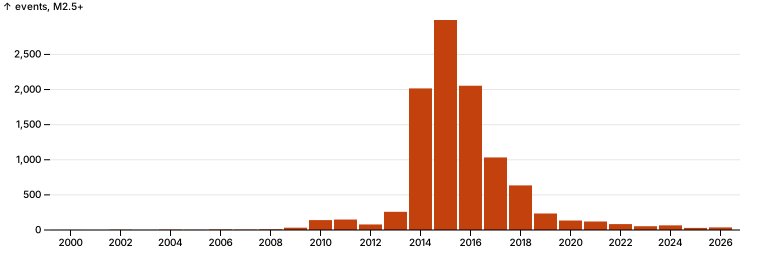
The raw count first: every event of magnitude 2.5 and up in the area, by year. Later sections test whether this count means the same thing in every year.

import * as pl from "npm:nodejs-polars@0.18.0";
import * as Plot from "npm:@observablehq/plot@0.6.17";
import { parseHTML } from "npm:linkedom@0.18.9";
import { catalog, md } from "./quakes.ts";

const { document } = parseHTML("<html></html>");
const raw = catalog();
const counts = Object.fromEntries(raw.groupBy("year").agg(pl.col("id").count().alias("n")).toRecords().map((r) => [r.year, r.n]));
// Every year, including ones with no events (2001), so the axis is even.
const perYear = Array.from({ length: 27 }, (_, i) => ({ year: 2000 + i, events: counts[2000 + i] ?? 0 }));

Plot.plot({
  document, width: 760, height: 260, marginLeft: 50,
  x: { label: null, tickFormat: "d", ticks: perYear.filter((d) => d.year % 2 === 0).map((d) => d.year) },
  y: { grid: true, label: "events, M2.5+" },
  marks: [Plot.barY(perYear, { x: "year", y: "events", fill: "#c2410c" }), Plot.ruleY([0])],
})

const peak = perYear.reduce((a, b) => (b.events > a.events ? b : a));
const at = (y: number) => perYear.find((d) => d.year === y)!.events;
jupyter.md`| | events |
|---|---|
| 2000–2008, per year | ${(perYear.filter((d) => d.year <= 2008).reduce((s, d) => s + d.events, 0) / 9).toFixed(1)} |
| peak (${peak.year}) | ${peak.events.toLocaleString()} |
| 2024 | ${at(2024)} |
| 2025 | ${at(2025)} |
| 2026 (Jan–Oct) | ${at(2026)} |
| 2025 vs peak | ${((at(2025) / peak.events - 1) * 100).toFixed(1)}% |`

	events
2000–2008, per year	4.1
peak (2015)	2,990
2024	66
2025	30
2026 (Jan–Oct)	37
2025 vs peak	-99.0%

Finding (revised after section 3). The boom is over: 2,990 events of M2.5+ in 2015, about 56 in 2025 on a consistent magnitude scale (−98%). The published count of 30, which made 2025 look like the quietest year since 2009, is partly a change of network (section 3); on one scale the rate has been flat since 2023. It is not back to before the boom: 2000–2008 averaged 4.1 a year, so 2025 is still about 14 times that.

2. Is every year measured the same way?

The catalog merges solutions from several networks, each with its own magnitude scale. If the network or the scale changed over the years, the yearly counts compare different things. Two columns say: net (who located the event and set the preferred magnitude) and magType (the scale). Also check type, since the catalog holds more than earthquakes.

const byYear = (col: string) =>
  raw.groupBy(["year", col]).agg(pl.col("id").count().alias("n"))
     .pivot("n", { index: "year", on: col }).fillNull("zero").sort("year");
// Pivot columns come out in hash order; fix it so the table is the same on every run.
const sorted = (df: pl.DataFrame) => df.select("year", ...df.columns.filter((c) => c !== "year").sort());

md(byYear("net").filter(pl.col("year").gtEq(2012)))

year	ok	us	ismpkansas
2012	0	79	0
2013	0	259	0
2014	0	1,985	31
2015	0	2,946	44
2016	0	2,054	0
2017	0	1,033	0
2018	0	635	0
2019	144	91	0
2020	128	7	0
2021	115	6	0
2022	78	6	0
2023	53	1	0
2024	65	1	0
2025	26	4	0
2026	36	1	0

md(sorted(byYear("magType")).filter(pl.col("year").gtEq(2008)))

year	mb	mb_lg	mblg	md	ml	mwc	mwr	mww
2008	0	0	5	5	0	0	0	0
2009	0	0	33	0	0	0	0	0
2010	0	0	53	76	0	1	11	0
2011	0	0	17	57	64	0	10	1
2012	1	0	9	0	67	0	2	0
2013	0	10	12	0	227	0	10	0
2014	0	117	0	0	1,767	0	131	1
2015	2	202	0	0	2,619	0	167	0
2016	3	84	0	0	1,862	0	101	4
2017	0	131	0	0	857	0	45	0
2018	1	60	0	0	546	0	26	2
2019	0	75	0	0	147	0	13	0
2020	0	6	0	0	126	0	3	0
2021	0	5	0	0	112	0	4	0
2022	0	5	0	0	78	0	0	1
2023	0	1	0	0	52	0	1	0
2024	0	0	0	0	62	0	3	1
2025	0	4	0	0	26	0	0	0
2026	0	1	0	0	35	0	1	0

// Earthquakes only, from here on.
const quakes = raw.filter(pl.col("type").eq(pl.lit("earthquake")));
md(raw.filter(pl.col("type").neq(pl.lit("earthquake"))).select("time", "mag", "type", "place"), 2)

time	mag	type	place
2020-01-11T13:00:56.700Z	2.82	other event	13 km WNW of Wilson, Oklahoma
2022-07-20T16:43:10.470Z	2.51	quarry blast	9 km WSW of Lebanon, Oklahoma

Finding. The rows are not measured the same way across the years.

• Who sets the magnitude changed in 2019. Through 2018 almost every preferred solution is USGS's (us). From 2019 it is the Oklahoma Geological Survey's (ok): 144 of 235 events that year, and 26 of 30 in 2025.
• Both use local magnitude (ml), but each network computes it from its own stations and calibration. The same label does not guarantee the same number for the same quake. These rows alone can't say whether the two agree.
• mblg and mb_lg are one scale spelled two ways (the spelling changes in 2013); not a real change.
• Two rows are not earthquakes (a quarry blast in 2022, an "other event" in 2020). Dropped from here on as quakes.

So the drop after 2019 mixes a real change with a change of network. The size of the second is still unknown.

Recorded: ran in the shell, not in this kernel.

$ Q="format=csv&starttime=2019-01-01&endtime=2026-11-01&minlatitude=33.6&maxlatitude=37.5&minlongitude=-100&maxlongitude=-94.4&minmagnitude=1.5&orderby=time-asc"; for net in us ok; do curl -sSfo data/$net-m15.csv "https://earthquake.usgs.gov/fdsnws/event/1/query?$Q&catalog=$net"; done; wc -l data/us-m15.csv data/ok-m15.csv

   1884 data/us-m15.csv
   9144 data/ok-m15.csv
  11028 total

3. Do USGS and OGS give the same quake the same magnitude?

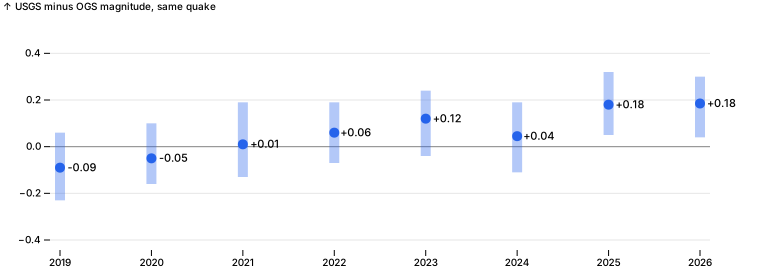
ComCat keeps each network's own solution, not only the preferred one. Both catalogs from 2019 on, down to M1.5 so events near the 2.5 cut still find their partner (recorded above). An event in both is the same quake when the origin times are within 8 seconds and the epicentres within 15 km. The difference that matters is USGS minus OGS for the same quake: positive means OGS reads lower.

import { match } from "./quakes.ts";

const usCat = catalog("../data/us-m15.csv").filter(pl.col("type").eq(pl.lit("earthquake")));
const okCat = catalog("../data/ok-m15.csv").filter(pl.col("type").eq(pl.lit("earthquake")));
const pairs = pl.DataFrame(match(usCat.toRecords(), okCat.toRecords()))
  .withColumns(pl.col("magA").minus(pl.col("magB")).alias("diff"));

[usCat.height, okCat.height, pairs.height]

[ 1881, 8353, 1566 ]

const offset = pairs.groupBy("year").agg(
  pl.col("diff").count().alias("pairs"),
  pl.col("diff").quantile(0.25).alias("q25"),
  pl.col("diff").median().alias("median"),
  pl.col("diff").quantile(0.75).alias("q75"),
).sort("year");
md(offset, 2)

year	pairs	q25	median	q75
2019	293.00	-0.23	-0.09	0.06
2020	266.00	-0.16	-0.05	0.10
2021	250.00	-0.13	0.01	0.19
2022	183.00	-0.07	0.06	0.19
2023	169.00	-0.04	0.12	0.24
2024	170.00	-0.11	0.04	0.19
2025	137.00	0.05	0.18	0.32
2026	98.00	0.04	0.18	0.30

Plot.plot({
  document, width: 760, height: 280, marginLeft: 50, marginRight: 50, inset: 10,
  x: { label: null, tickFormat: "d", ticks: offset.getColumn("year").toArray() },
  y: { grid: true, label: "USGS minus OGS magnitude, same quake", domain: [-0.4, 0.5] },
  marks: [
    Plot.ruleY([0], { stroke: "#888" }),
    Plot.ruleX(offset.toRecords(), { x: "year", y1: "q25", y2: "q75", stroke: "#2563eb", strokeWidth: 10, strokeOpacity: 0.35 }),
    Plot.dot(offset.toRecords(), { x: "year", y: "median", r: 5, fill: "#2563eb" }),
    Plot.text(offset.toRecords(), { x: "year", y: "median", text: (d) => (d.median >= 0 ? "+" : "") + d.median.toFixed(2), dx: 22, fontSize: 11 }),
  ],
})

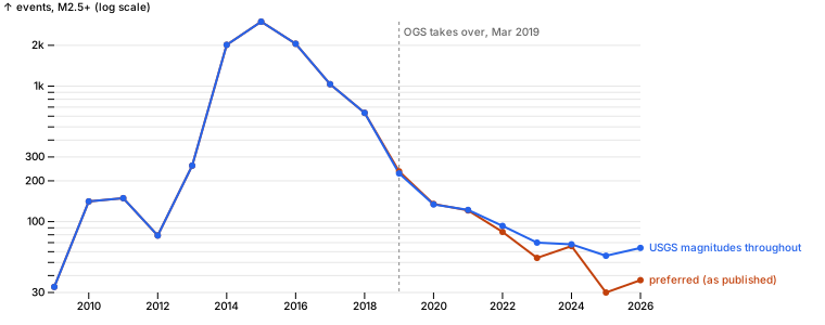
// Events of M2.5+ per year as each network measures them, next to the preferred (merged) count.
const m25 = (df: pl.DataFrame, name: string) =>
  df.filter(pl.col("mag").gtEq(2.5)).groupBy("year").agg(pl.col("id").count().alias(name));
const scales = m25(quakes.filter(pl.col("year").gtEq(2019)), "preferred")
  .join(m25(usCat, "usgs"), { on: "year" })
  .join(m25(okCat, "ogs"), { on: "year" })
  .sort("year");
md(scales)

year	preferred	usgs	ogs
2019	235	227	144
2020	134	134	127
2021	121	122	115
2022	83	93	77
2023	54	70	53
2024	66	68	65
2025	30	56	26
2026	37	64	36

// When do OGS solutions start? Events per month in the OGS catalog, 2019.
md(okCat.filter(pl.col("year").eq(2019)).groupBy(pl.col("time").str.slice(0, 7).alias("month")).agg(pl.col("id").count().alias("ogs_events")).sort("month"))

month	ogs_events
2019-03	107
2019-04	54
2019-05	14
2019-06	170
2019-07	259
2019-08	201
2019-09	143
2019-10	144
2019-11	164
2019-12	137

// One series on USGS's own magnitudes for every year: the preferred count through 2018 (all but 75 of those events are USGS's), the USGS catalog from 2019.
const usgsByYear = Object.fromEntries(scales.toRecords().map((r) => [r.year, r.usgs]));
const series = perYear.filter((d) => d.year >= 2009).flatMap((d) => [
  { year: d.year, events: d.events, series: "preferred (as published)" },
  { year: d.year, events: d.year >= 2019 ? usgsByYear[d.year] : d.events, series: "USGS magnitudes throughout" },
]);
Plot.plot({
  document, width: 760, height: 300, marginLeft: 50, marginRight: 170,
  x: { label: null, tickFormat: "d" },
  y: { type: "log", grid: true, label: "events, M2.5+ (log scale)" },
  color: { domain: ["preferred (as published)", "USGS magnitudes throughout"], range: ["#c2410c", "#2563eb"] },
  marks: [
    Plot.ruleX([2019], { stroke: "#888", strokeDasharray: "3,3" }),
    Plot.text([{ x: 2019, y: 2500 }], { x: "x", y: "y", text: () => "OGS takes over, Mar 2019", textAnchor: "start", dx: 4, fill: "#666" }),
    Plot.line(series, { x: "year", y: "events", stroke: "series", strokeWidth: 2 }),
    Plot.dot(series, { x: "year", y: "events", fill: "series", r: 3 }),
    Plot.text(series.filter((d) => d.year === 2026), { x: "year", y: "events", text: "series", fill: "series", textAnchor: "start", dx: 8 }),
  ],
})

Finding. OGS has been reading lower than USGS for the same quake, and the gap is growing. In 2019 OGS read 0.09 higher (median of 293 matched quakes); by 2025–2026 it reads 0.18 lower. Near the 2.5 cut, a few tenths of a magnitude decide whether a quake is counted at all.

On USGS's own magnitudes, 2025 had 56 events of M2.5+, not 30, and 2026 has 64 through October, not 37. The published series makes 2025 look like a new low; on one scale the rate has been flat at about 55–70 a year since 2023. The steep fall from 2015 to 2021 is real on either scale.

(2019 differs the other way only because OGS solutions start in March 2019.)

4. Mainshocks or aftershocks?

A swarm year counts every aftershock. Separate them with the standard Gardner–Knopoff (1974) windows: a quake of magnitude m claims smaller quakes within a distance and time that grow with m (M3: 22 km, 12 days; M4: 30 km, 41 days; M5.8 Pawnee: 49 km, 391 days). What is left, the mainshocks, is the rate of independent quakes: the background the question is really about. decluster() in quakes.ts.

import { decluster } from "./quakes.ts";

const dep = decluster(quakes.toRecords());
const labelled = quakes.withColumns(pl.Series("kind", dep.map((d) => (d ? "aftershock" : "mainshock"))));
const kinds = labelled.groupBy("year").agg(
  pl.col("id").count().alias("all"),
  pl.col("kind").eq(pl.lit("mainshock")).sum().alias("mainshocks"),
).withColumns(pl.col("mainshocks").cast(pl.Float64).div(pl.col("all")).mul(100).alias("mainshock_pct")).sort("year");
md(kinds.filter(pl.col("year").gtEq(2009)))

year	all	mainshocks	mainshock_pct
2009	33	17	52
2010	141	38	27
2011	149	22	15
2012	79	19	24
2013	259	62	24
2014	2,016	174	9
2015	2,990	201	7
2016	2,054	165	8
2017	1,033	217	21
2018	635	207	33
2019	235	117	50
2020	134	75	56
2021	121	64	53
2022	83	47	57
2023	54	34	63
2024	66	34	52
2025	30	23	77
2026	37	23	62

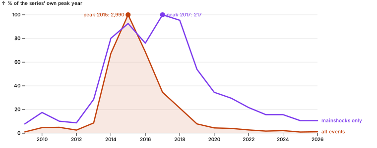
// Each series as a share of its own peak year, so their shapes can be compared.
const k = kinds.filter(pl.col("year").gtEq(2009)).toRecords();
const peakAll = Math.max(...k.map((d) => d.all)), peakMain = Math.max(...k.map((d) => d.mainshocks));
const shapes = k.flatMap((d) => [
  { year: d.year, share: d.all / peakAll, n: d.all, series: "all events" },
  { year: d.year, share: d.mainshocks / peakMain, n: d.mainshocks, series: "mainshocks only" },
]);
Plot.plot({
  document, width: 760, height: 300, marginLeft: 50, marginRight: 120, marginTop: 30,
  x: { label: null, tickFormat: "d" },
  y: { grid: true, percent: true, label: "% of the series' own peak year" },
  color: { domain: ["all events", "mainshocks only"], range: ["#c2410c", "#7c3aed"] },
  marks: [
    Plot.areaY(shapes.filter((d) => d.series === "all events"), { x: "year", y: "share", fill: "#c2410c", fillOpacity: 0.12 }),
    Plot.line(shapes, { x: "year", y: "share", stroke: "series", strokeWidth: 2.5 }),
    Plot.dot(shapes.filter((d) => d.share === 1), { x: "year", y: "share", fill: "series", r: 5 }),
    Plot.text(shapes.filter((d) => d.share === 1 && d.series === "all events"), { x: "year", y: "share", text: (d) => `peak ${d.year}: ${d.n.toLocaleString()}`, dx: -8, textAnchor: "end", fill: "series" }),
    Plot.text(shapes.filter((d) => d.share === 1 && d.series === "mainshocks only"), { x: "year", y: "share", text: (d) => `peak ${d.year}: ${d.n}`, dx: 8, textAnchor: "start", fill: "series" }),
    Plot.text(shapes.filter((d) => d.year === 2026), { x: "year", y: "share", text: "series", fill: "series", textAnchor: "start", dx: 8 }),
  ],
})

// Baseline and recent mainshock rates, for the finding below.
const ks = kinds.toRecords();
jupyter.md`| | mainshocks per year |
|---|---|
| 2000–2008 average | ${(ks.filter((d) => d.year <= 2008).reduce((s, d) => s + d.mainshocks, 0) / 9).toFixed(1)} |
${ks.filter((d) => d.year >= 2023).map((d) => `| ${d.year} | ${d.mainshocks} |`).join("\n")}`

	mainshocks per year
2000–2008 average	3.6
2023	34
2024	34
2025	23
2026	23

Finding. Most of the boom's count was aftershocks, and independent quakes peaked two years later than the count did.

• In 2015, only 201 of 2,990 events (7%) were mainshocks. The rest belonged to sequences.
• Mainshocks peaked in 2017 (217), not 2015. The fall in the raw count from 2015 to 2017 (−65%) was fewer aftershocks; independent quakes were still rising, after the 2015–2016 injection cuts had begun.
• From 2017 to 2025 mainshocks fell 89% (217 to 23). Since 2023 they run at 23–34 a year, about 6–10 times the 2000–2008 average of 3.6. These use the published magnitudes, so the recent years are slightly low (section 3).

So the background rate came down, but more slowly than the headline count, and it hasn't gone back to where it was.

5. Where are they?

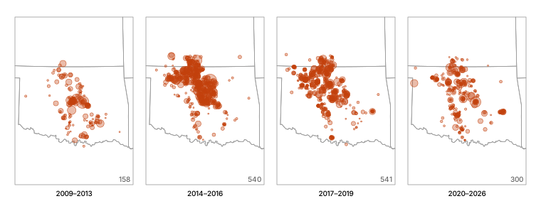
Mainshocks only (section 4), so a single aftershock sequence doesn't paint a region, in four eras: before the boom took off, the peak, the fall, and since. Dot size is magnitude. State lines from the US Census atlas (us-atlas).

import * as topo from "npm:topojson-client@3.1.0";
import us from "npm:us-atlas@3.0.1/states-10m.json" with { type: "json" };

const states = topo.feature(us, us.objects.states);
const near = { type: "FeatureCollection", features: states.features.filter((f) => ["Oklahoma", "Kansas", "Texas", "Arkansas", "Missouri"].includes(f.properties.name)) };
const box = { type: "MultiPoint", coordinates: [[-100, 33.6], [-94.4, 37.5], [-100, 37.5], [-94.4, 33.6]] };
const era = (y: number) => (y < 2014 ? "2009–2013" : y < 2017 ? "2014–2016" : y < 2020 ? "2017–2019" : "2020–2026");
const mains = labelled.filter(pl.col("kind").eq(pl.lit("mainshock"))).filter(pl.col("year").gtEq(2009))
  .toRecords().map((d) => ({ ...d, era: era(d.year) }));

Plot.plot({
  document, width: 760, height: 290, marginTop: 24,
  projection: { type: "conic-equal-area", parallels: [34, 37], rotate: [97.2, 0], domain: box, inset: 4 },
  fx: { label: null, domain: ["2009–2013", "2014–2016", "2017–2019", "2020–2026"] },
  r: { range: [1, 9], domain: [2.5, 5.8] },
  marks: [
    Plot.geo(near, { stroke: "#999", strokeWidth: 0.8 }),
    Plot.dot(mains, { x: "lon", y: "lat", r: "mag", fx: "era", fill: "#c2410c", fillOpacity: 0.35, stroke: "#c2410c", strokeWidth: 0.5 }),
    Plot.text(mains, Plot.groupZ({ text: "count" }, { fx: "era", frameAnchor: "bottom-right", dy: -4, dx: -4, text: (d) => d, fill: "#666" })),
  ],
})

// How far north: share of mainshocks above 36.5° N (north-central Oklahoma and the Kansas border), by year.
const north = pl.DataFrame(mains).groupBy("year").agg(
  pl.col("id").count().alias("mainshocks"),
  pl.col("lat").mean().alias("mean_lat"),
  pl.col("lat").gtEq(36.5).cast(pl.Float64).mean().mul(100).alias("pct_north_of_36_5"),
).sort("year");
md(north, 1)

year	mainshocks	mean_lat	pct_north_of_36_5
2009	17.0	35.5	0.0
2010	38.0	35.1	2.6
2011	22.0	35.1	0.0
2012	19.0	35.4	5.3
2013	62.0	35.6	21.0
2014	174.0	36.2	39.7
2015	201.0	36.3	40.8
2016	165.0	36.2	38.2
2017	217.0	36.3	35.9
2018	207.0	36.2	33.3
2019	117.0	35.9	27.4
2020	75.0	36.2	32.0
2021	64.0	35.8	25.0
2022	47.0	35.9	31.9
2023	34.0	35.8	17.6
2024	34.0	35.8	11.8
2025	23.0	35.9	21.7
2026	23.0	35.3	0.0

Finding. The activity did move north and come back, partly.

• Before 2013, almost no mainshocks were north of 36.5° N. From 2014 to 2018, 33–41% were, along the Kansas border (the dense clusters in the 2014–2016 and 2017–2019 maps).
• Since 2023 that share is 12–22% (0 of 23 so far in 2026), and the average latitude is 35.8–35.9°, south of the 36.2–36.3° of 2014–2018 but still north of 2009–2013 (35.1–35.6°).
• What remains is a band from north-central Oklahoma down through the center of the state, overlapping the area of the 2009–2013 activity but reaching further north.

6. One town: Stillwater

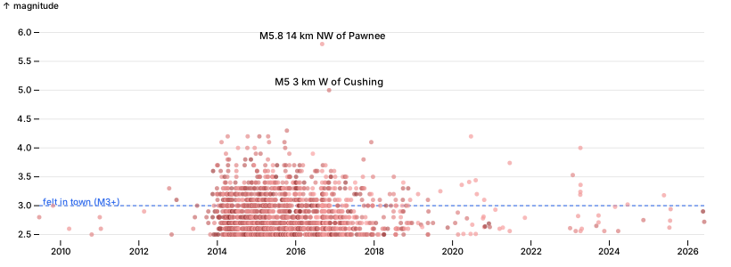
Thomas added the two cells below: the question, and the town with a 40 km radius. Using them as given: every quake within town.radiusKm of the town, and those of M3+, which people in town would usually feel. All events here, aftershocks included, since an aftershock shakes the house just the same.

Thomas: what has this been like in one town? Stillwater is between the Pawnee and Cushing quakes. Count quakes within 40 km of town by year, and the ones people would have felt (M3+).

const town = { name: "Stillwater", lat: 36.1156, lon: -97.0584, radiusKm: 40 };

import { km } from "./quakes.ts";

const local = quakes.toRecords()
  .map((d) => ({ ...d, dist: km(town.lat, town.lon, d.lat, d.lon) }))
  .filter((d) => d.dist <= town.radiusKm);
const localYears = Array.from({ length: 2026 - 2009 + 1 }, (_, i) => 2009 + i).map((year) => {
  const ys = local.filter((d) => d.year === year);
  return { year, events: ys.length, felt_m3: ys.filter((d) => d.mag >= 3).length, largest: ys.length ? Math.max(...ys.map((d) => d.mag)).toFixed(1) : "–" };
});
md(pl.DataFrame(localYears))

year	events	felt_m3	largest
2009	2	1	3.0
2010	2	0	2.6
2011	2	0	2.8
2012	4	2	3.3
2013	20	7	3.7
2014	631	180	4.2
2015	649	209	4.3
2016	464	131	5.8
2017	154	45	4.1
2018	55	18	3.5
2019	12	3	3.3
2020	20	6	4.2
2021	6	1	3.7
2022	1	0	2.6
2023	13	5	4.0
2024	4	1	3.0
2025	4	1	3.2
2026	2	0	2.9

// Every quake within the radius, 2009 on: when, how big, how far from town (darker = closer).
const notable = local.filter((d) => d.mag >= 4.5);
Plot.plot({
  document, width: 820, height: 300, marginLeft: 44, marginRight: 30, marginTop: 30,
  x: { type: "utc", label: null },
  y: { grid: true, label: "magnitude", domain: [2.4, 6.1] },
  color: { type: "linear", domain: [0, 40], range: ["#7f1d1d", "#fca5a5"], legend: false },
  marks: [
    Plot.ruleY([3], { stroke: "#2563eb", strokeDasharray: "4,3" }),
    Plot.text(["felt in town (M3+)"], { frameAnchor: "top-left", y: 3, dy: -8, dx: 4, fill: "#2563eb", textAnchor: "start" }),
    Plot.dot(local.filter((d) => d.year >= 2009), { x: (d) => new Date(d.time), y: "mag", r: 2.5, fill: "dist", fillOpacity: 0.7 }),
    Plot.text(notable, { x: (d) => new Date(d.time), y: "mag", text: (d) => `M${d.mag} ${d.place.replace(/, Oklahoma$/, "")}`, dy: -9, fontSize: 11 }),
  ],
})

// The felt quakes since 2021, for the finding below.
md(pl.DataFrame(local.filter((d) => d.year >= 2021 && d.mag >= 3).map((d) => ({ date: d.time.slice(0, 10), mag: d.mag, place: d.place, km_from_town: d.dist }))), 1)

date	mag	place	km_from_town
2021-06-16	3.7	3 km SE of Carney, Oklahoma	36.6
2023-01-25	3.5	5 km ENE of Meridian, Oklahoma	31.7
2023-04-05	3.2	4 km ESE of Carney, Oklahoma	36.6
2023-04-06	4.0	4 km ESE of Carney, Oklahoma	36.7
2023-04-06	3.2	Oklahoma	36.7
2023-04-07	3.4	3 km ESE of Carney, Oklahoma	36.8
2024-06-19	3.0	11 km E of Red Rock, Oklahoma	36.7
2025-05-23	3.2	11 km NW of Pawnee, Oklahoma	37.3

Finding. In Stillwater the boom was a daily experience and is now an occasional one.

• 2014–2016: 1,744 quakes within 40 km, 520 of them M3+: a quake people would feel about every two days for three years, plus the two largest in the record, M5.8 Pawnee (Sep 2016, 37 km away) and M5.0 Cushing (Nov 2016).
• 2021 to October 2026: 8 felt quakes in almost six years, 4 of them in a three-day sequence near Carney in April 2023 (largest M4.0, 37 km away).
• 2009–2012: three felt quakes in four years.

The town is close to its pre-boom experience, though not at it, and on USGS's scale (section 3) the recent counts would be a little higher.

7. Are the big ones falling as fast as the count?

Damage comes from the rare large quakes, so the question is whether the share of large ones changed. Two ways to look:

1. M4+ per year, next to all events. Few, so read them by era, not by year.
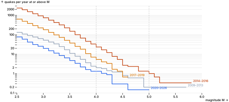
2. The Gutenberg–Richter slope (b-value). Counts fall about tenfold per magnitude unit; b is that slope. A lower b means a larger share of big quakes. Maximum-likelihood estimate (Aki 1965) above M2.5, with its standard error b/√n. Eras as in section 5.

const eraOf = (y: number) => (y < 2009 ? null : era(y));
const eraStats = ["2009–2013", "2014–2016", "2017–2019", "2020–2026"].map((name) => {
  const m = quakes.toRecords().filter((d) => eraOf(d.year) === name).map((d) => d.mag);
  const mean = m.reduce((s, v) => s + v, 0) / m.length;
  const b = Math.LOG10E / (mean - (2.5 - 0.05));
  return {
    era: name, events: m.length, m4: m.filter((v) => v >= 4).length,
    per_1000: (1000 * m.filter((v) => v >= 4).length) / m.length,
    b, b_se: b / Math.sqrt(m.length),
  };
});
md(pl.DataFrame(eraStats), 2)

era	events	m4	per_1000	b	b_se
2009–2013	661.00	10.00	15.13	0.93	0.04
2014–2016	7,060.00	70.00	9.92	1.07	0.01
2017–2019	1,903.00	16.00	8.41	1.16	0.03
2020–2026	525.00	9.00	17.14	1.10	0.05

// Gutenberg–Richter: quakes per year at or above each magnitude, one line per era.
const eraYears = { "2009–2013": 5, "2014–2016": 3, "2017–2019": 3, "2020–2026": 6 + 10 / 12 };
const grid = Array.from({ length: 34 }, (_, i) => +(2.5 + i * 0.1).toFixed(1));
const gr = Object.entries(eraYears).flatMap(([name, years]) => {
  const m = quakes.toRecords().filter((d) => eraOf(d.year) === name).map((d) => d.mag);
  return grid.map((M) => ({ era: name, M, perYear: m.filter((v) => v >= M - 1e-9).length / years })).filter((d) => d.perYear > 0);
});
Plot.plot({
  document, width: 760, height: 340, marginLeft: 56, marginRight: 90,
  x: { label: "magnitude M", domain: [2.5, 6] },
  y: { type: "log", grid: true, label: "quakes per year at or above M", tickFormat: "~g", domain: [0.1, 3000] },
  color: { domain: Object.keys(eraYears), range: ["#94a3b8", "#c2410c", "#d97706", "#2563eb"] },
  marks: [
    Plot.line(gr, { x: "M", y: "perYear", stroke: "era", strokeWidth: 2, curve: "step-after" }),
    Plot.text(gr, Plot.selectLast({ x: "M", y: "perYear", z: "era", text: "era", fill: "era", textAnchor: "start", dx: 6, dy: -6 })),
    Plot.ruleX([4, 5], { stroke: "#aaa", strokeDasharray: "3,3" }),
  ],
})

// Every M4.5+ quake, for the finding below.
md(quakes.filter(pl.col("mag").gtEq(4.5)).select(pl.col("time").str.slice(0, 10).alias("date"), "mag", "place").sort("date"), 2)

date	mag	place
2011-11-05	4.80	8 km SE of Sparks, Oklahoma
2011-11-06	5.70	8 km NW of Prague, Oklahoma
2011-11-08	4.80	9 km SSE of Sparks, Oklahoma
2013-12-07	4.50	8 km SW of Arcadia, Oklahoma
2014-11-12	4.90	4 km ENE of Milan, Kansas
2015-07-27	4.50	4 km NNE of Crescent, Oklahoma
2015-11-19	4.70	4 km SW of Lambert, Oklahoma
2015-11-30	4.70	8 km E of Nescatunga, Oklahoma
2016-01-07	4.70	16 km SE of Waynoka, Oklahoma
2016-02-13	5.10	18 km SE of Waynoka, Oklahoma
2016-09-03	5.80	14 km NW of Pawnee, Oklahoma
2016-11-07	5.00	3 km W of Cushing, Oklahoma
2018-04-07	4.60	5 km WNW of Lucien, Oklahoma
2018-04-09	4.60	8 km NNE of Marshall, Oklahoma
2022-01-31	4.50	7 km NW of Medford, Oklahoma
2024-02-03	5.06	8 km NW of Prague, Oklahoma

Finding. The risk of a large quake fell about as fast as the count: not faster, and not measurably slower.

• The whole curve moved down. The mix of sizes did shift some: b rose from 1.07 at the peak to 1.16 in 2017–2019 (fewer large quakes per event as the rate fell) and is 1.10 since 2020, the same as the peak within its error. 2009–2013 had the largest share of big quakes (b 0.93). The b estimates assume magnitudes rounded to 0.1; OGS reports two decimals, which would lower the 2020–2026 b by up to 0.1 (to about 1.0), so the recent mix may hold slightly more large quakes than the peak's. M4+ ran at 23 a year in 2014–2016, 5.3 in 2017–2019 and 1.3 since 2020, below 2009–2013 (2 a year).
• 2020–2026 has more M4+ per 1,000 events (17) than the peak (10), but that is 9 quakes. A Poisson 95% range for 9 is 4 to 17, or 8 to 33 per 1,000, which includes the peak's rate. OGS's lower magnitudes (section 3) also shrink the denominator.
• Pawnee (M5.8, Sep 2016) came when the raw count was falling but mainshocks were still near their peak (section 4). That is the series to watch for large-quake risk, not the headline count.
• Large quakes have not stopped: M5.06 near Prague in February 2024 (table above).

Recorded: ran in the shell, not in this kernel.

$ mkdir -p data/occ && for y in $(seq 2011 2025); do curl -sSfLo data/occ/$y.xlsx "https://oklahoma.gov/content/dam/ok/en/occ/documents/og/ogdatafiles/$y-uic-injection-volumes.xlsx"; done; ls data/occ | wc -l; du -sh data/occ

15
51M	data/occ

8. Does injection line up with the quakes?

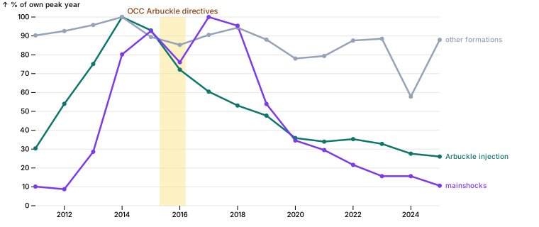
The catalog alone can't show cause. The Oklahoma Corporation Commission publishes every disposal well's monthly injection volume (Form 1012), 2011–2025 (recorded above). Disposal into the deep Arbuckle group, close to the basement faults, is the injection linked to the quakes; the OCC's 2015–2016 directives cut Arbuckle volumes in the quake areas. Wells inside the study area only. This can show whether timing and place line up, not prove cause.

import { injection } from "./quakes.ts";

const inj = (await injection(Array.from({ length: 15 }, (_, i) => 2011 + i)))
  .filter(pl.col("lat").gtEq(33.6).and(pl.col("lat").ltEq(37.5)).and(pl.col("lon").gtEq(-100)).and(pl.col("lon").ltEq(-94.4)));
[inj.height, inj.select(pl.col("api").nUnique()).row(0)[0]]

[ 1284694, 11378 ]

// Sanity check before summing: the largest single well-month volumes.
md(inj.sort("barrels", true).head(8).select("year", "month", "api", "formation", "barrels"))

year	month	api	formation	barrels
2020	2	3507324320	OSWEGO	10,009,670
2020	8	3507324320	OSWEGO	8,935,046
2024	2	3504322287	LOWER MORROW SAND	8,300,091
2020	1	3513325025	ARBUCKLE	5,158,248
2020	12	3501520306	PONTOTOC	4,876,145
2018	1	3513726796	LOCO SAND	LOCO SD
2018	2	3513726796	LOCO SAND	LOCO SD
2018	3	3513726796	LOCO SAND	LOCO SD

// The numbers behind the cut-off below.
const q999 = inj.filter(pl.col("arbuckle")).select(pl.col("barrels").quantile(0.999)).row(0)[0];
jupyter.md`| | |
|---|---|
| well-month rows in the area | ${inj.height.toLocaleString()} |
| Arbuckle well-months, 99.9th percentile | ${Math.round(q999).toLocaleString()} barrels |
| well-months over 2 million barrels | ${inj.filter(pl.col("barrels").gt(2_000_000)).height} |`

well-month rows in the area	1,284,694
Arbuckle well-months, 99.9th percentile	1,107,043 barrels
well-months over 2 million barrels	43

Data check. Some reports are not believable: one shallow Oswego well reports 10 million barrels in a month (330,000 a day), and another repeats 4.0 million every month of 2018. The busiest Arbuckle wells top out near 1.1 million a month (99.9th percentile). Well-months over 2 million barrels are dropped as entry errors: 43 of 1.28 million rows.

const injOk = inj.filter(pl.col("barrels").ltEq(2_000_000));
const injYear = injOk.groupBy("year").agg(
  pl.col("barrels").filter(pl.col("arbuckle")).sum().div(1e6).alias("arbuckle_mbbl"),
  pl.col("barrels").filter(pl.col("arbuckle").not()).sum().div(1e6).alias("other_mbbl"),
  pl.col("api").filter(pl.col("arbuckle")).nUnique().alias("arbuckle_wells"),
).sort("year");
md(injYear)

year	arbuckle_mbbl	other_mbbl	arbuckle_wells
2011	252	1,604	290
2012	448	1,646	424
2013	623	1,703	531
2014	829	1,778	614
2015	771	1,590	583
2016	598	1,515	587
2017	501	1,609	556
2018	440	1,677	538
2019	396	1,565	519
2020	297	1,387	459
2021	282	1,410	423
2022	293	1,556	408
2023	272	1,573	402
2024	229	1,028	368
2025	216	1,563	371

// Arbuckle injection, injection into everything else, and mainshocks, each as % of its own peak year.
const mainsByYear = Object.fromEntries(kinds.toRecords().map((r) => [r.year, r.mainshocks]));
const iy = injYear.toRecords();
const pk = (k: string) => Math.max(...iy.map((d) => d[k]));
const peakM = Math.max(...iy.map((d) => mainsByYear[d.year]));
const timing = iy.flatMap((d) => [
  { year: d.year, share: d.arbuckle_mbbl / pk("arbuckle_mbbl"), series: "Arbuckle injection" },
  { year: d.year, share: d.other_mbbl / pk("other_mbbl"), series: "other formations" },
  { year: d.year, share: mainsByYear[d.year] / peakM, series: "mainshocks" },
]);
Plot.plot({
  document, width: 760, height: 320, marginLeft: 50, marginRight: 140, marginTop: 24,
  x: { label: null, tickFormat: "d" },
  y: { grid: true, percent: true, label: "% of own peak year", domain: [0, 100] },
  color: { domain: ["Arbuckle injection", "other formations", "mainshocks"], range: ["#0f766e", "#94a3b8", "#7c3aed"] },
  marks: [
    Plot.rectY([{ x1: 2015.3, x2: 2016.2 }], { x1: "x1", x2: "x2", y1: 0, y2: 1, fill: "#fde68a", fillOpacity: 0.5 }),
    Plot.text(["OCC Arbuckle directives"], { x: 2015.75, y: 1, dy: -8, fill: "#92400e", fontSize: 11 }),
    Plot.line(timing, { x: "year", y: "share", stroke: "series", strokeWidth: 2.5 }),
    Plot.dot(timing, { x: "year", y: "share", fill: "series", r: 3 }),
    Plot.text(timing.filter((d) => d.year === 2025), { x: "year", y: "share", text: "series", fill: "series", textAnchor: "start", dx: 8 }),
  ],
})

// Same comparison by place: north of 36.5° N (the Kansas-border cluster in section 5) and south of it.
const side = (lat: number) => (lat >= 36.5 ? "north" : "south");
const arbBySide = injOk.filter(pl.col("arbuckle")).withColumns(pl.col("lat").gtEq(36.5).alias("north"))
  .groupBy(["year", "north"]).agg(pl.col("barrels").sum().div(1e6).alias("mbbl")).toRecords();
const placeRows = [2013, 2014, 2015, 2016, 2017, 2018, 2019, 2021, 2023, 2025].map((year) => ({
  year,
  north_arbuckle_mbbl: arbBySide.find((d) => d.year === year && d.north)?.mbbl ?? 0,
  north_mainshocks: mains.filter((d) => d.year === year && side(d.lat) === "north").length,
  south_arbuckle_mbbl: arbBySide.find((d) => d.year === year && !d.north)?.mbbl ?? 0,
  south_mainshocks: mains.filter((d) => d.year === year && side(d.lat) === "south").length,
}));
md(pl.DataFrame(placeRows))

year	north_arbuckle_mbbl	north_mainshocks	south_arbuckle_mbbl	south_mainshocks
2013	409	13	214	49
2014	498	69	332	105
2015	479	82	292	119
2016	347	63	251	102
2017	276	78	225	139
2018	221	69	219	138
2019	187	32	209	85
2021	119	16	163	48
2023	105	6	167	28
2025	78	5	139	18

// Wells with a location reporting non-Arbuckle volumes, by year: checks the 2024 dip.
md(injOk.filter(pl.col("arbuckle").not()).groupBy("year").agg(pl.col("api").nUnique().alias("located_wells"), pl.col("barrels").sum().div(1e6).alias("mbbl")).sort("year").filter(pl.col("year").gtEq(2020)))

year	located_wells	mbbl
2020	6,972	1,387
2021	6,827	1,410
2022	6,867	1,556
2023	6,761	1,573
2024	5,030	1,028
2025	6,407	1,563

Finding. Timing and place line up with Arbuckle injection, and not with injection in general.

• Arbuckle volumes in the area tripled from 2011 to 2014 (252 to 829 million barrels), then fell every year to 216 million in 2025 (−74%). Injection into other formations stayed at 1.4–1.7 billion barrels most years, with no trend; quakes did not follow it.
• Mainshocks rose behind the Arbuckle rise and peaked in 2017, three years after Arbuckle volumes peaked (2014). They have fallen with them since 2019, and a little faster.
• By place, 2015 to 2025: north of 36.5° N, where the cuts were deepest, Arbuckle fell 84% (479 to 78 million barrels) and mainshocks 94% (82 to 5). South of it, Arbuckle fell 52% (292 to 139) and mainshocks 85% (119 to 18). North's share of quakes shrank as its injection did (section 5).

What this does not show: mechanism. This notebook shows coincidence in time and place. The physical case, that pressure from Arbuckle disposal spreads to basement faults with a delay, is made elsewhere, not tested here: Keranen et al. 2014, Science 345:448; Langenbruch & Zoback 2016, Science Advances 2:e1601542.

Open: the 2024 dip in other-formation volume (1.03 billion) is a reporting gap: about 1,700 fewer wells in the 2024 file have a location (5,030, against 6,400–6,900 in the years around it). 2024 Arbuckle may be slightly low for the same reason.