Tables and charts for TypeScript notebooks

A design note for #747: one call that shows a table, one that draws a chart, and later an sql tag over DuckDB. Thomas agreed the design on 2026-11-13, with each decision's recommendation (Decisions). cdp-kernel 0.11.0 has jupyter.table, jupyter.sql and jupyter.chart; cdp-kernel 0.12.0 adds paging through the kernel and the modules option the apps use to draw charts offline, and cdp-kernel 0.12.1 lets the apps run jupyter.sql offline too. #747 tracks the rest. The rest of this note is the design, updated where 0.12.0 changed it. Compared with Python checks it against what Python notebooks do.

The problem

A Python notebook shows a DataFrame as a table and a chart as a picture with no extra code. A TypeScript notebook on cdp-kernel does neither well:

• Tables. A Polars DataFrame shows as application/vnd.dataresource+json (50 rows), an HTML table of 10 rows and a one-line text summary (runtime/display.mjs). Nothing renders the first one: not the apps, not JupyterLab, not VS Code. An array of rows, an Arrow table or a DuckDB result shows as util.inspect text.
• Charts. Observable Plot needs a DOM, so on Node a cell imports linkedom and passes its document (the journal skill teaches this). A plot with a legend is a <figure> holding HTML and SVG, which shows as HTML: agents can't see it and ganymede nb publish frames it. A Vega-Lite spec shows as application/vnd.vegalite.v5+json, which the apps and the published page don't draw, so the example notebooks each carry their own vega.View(...).toSVG() helper.

The pieces exist: display.mjs already recognises Vega specs and Polars-style DataFrames and writes a text summary of a chart (#321). What's missing is one way in, and outputs every reader can show.

The proposal

Two calls on cdp-kernel's jupyter namespace, and a tag:

jupyter.table(rows);                    // array of rows, Arrow, Polars, DuckDB
jupyter.chart({ mark: "bar", ... });    // a Vega-Lite spec
jupyter.chart(Plot, { marks: [...] });  // Observable Plot options
const busy = await jupyter.sql`select * from trips where riders > ${min}`;

Each returns a value with a Symbol.for("Jupyter.display") method, as jupyter.md and jupyter.svg do, so it shows as the cell's result or through jupyter.display(). Every output is a MIME bundle the notebook already knows how to keep: the file stays valid .ipynb, the server learns nothing new, and other frontends show the fallbacks.

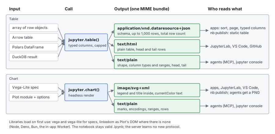
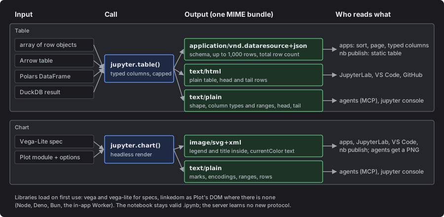
Table output

What it takes

jupyter.table(value, options?) accepts:

Input	Recognised by
An array of row objects	Array.isArray, objects in it
An array of arrays	with options.columns naming them
An Arrow table (apache-arrow, duckdb-wasm results)	schema.fields and numRows
A Polars DataFrame	the test display.mjs uses today
A DuckDB result from @duckdb/node-api	columnNames() and columnTypes()

The last three also show as a table when they are a cell's value, with no call, as Polars does today. A bare array keeps its inspect text unless passed to jupyter.table, so printing a list doesn't turn into a grid.

Options: columns (names, and order), limit (rows embedded, see The cap), title.

What it writes

One display_data with three parts:

• application/vnd.dataresource+json, the Table Schema bundle pandas, Polars and nteract already use: schema.fields with each column's name and type, and data as row objects. Ganymede adds one key the format allows, ganymede: { rows, shown }, with the total row count (when the source knows it) and how many rows are embedded.
• text/html, a plain <table> with each column's type under its name: up to 20 rows, and past that the first 10 and the last 5 with a "… N more rows" line between. JupyterLab, VS Code and GitHub show this. It has no styles or scripts, so it survives the sanitizer in an untrusted notebook.
• text/plain, for agents and jupyter console: the shape, each column's name, type and range (min and max, or distinct count, and nulls), and the first 3 and last 2 rows aligned as text, each row with its row number, so tail rows outside the embedded range show as such. It stays under 4 KB. Ranges come from the embedded rows, so for a cut table the summary says "ranges over the first 1,000 of 52,410 rows" rather than describing data it hasn't read.

Why not a new Ganymede MIME type: the data resource type already says what a table needs, other tools write it, and a later reader of it (the apps, nb publish) also shows tables from pandas notebooks. A Ganymede-only type would save nothing.

JSON rows, not Arrow IPC

The embedded rows are JSON. Arrow IPC would be base64 in a JSON file: larger after encoding, not readable in a diff or by an agent, and the apps would need the Arrow library to show it. With a cap on rows, JSON is small enough, and the kernel already holds Arrow tables only as a source to read from.

Values follow Table Schema types: integer and number as JSON numbers, except integers past 2^53 (bigint, Int64) as strings; NaN and infinities as the strings Table Schema allows; dates and times as ISO 8601 strings typed date, datetime or time; lists and structs as JSON typed array and object; binary as its length. A string over 1,000 characters is cut, with ….

The cap

By default the output embeds 1,000 rows, and stops earlier at 1 MB of JSON. limit raises it to 10,000 or lowers it. The footer and the summary always say "1,000 of 52,410 rows", so a cut table is never mistaken for the whole.

A cut table pages through the kernel (cdp-kernel 0.12.0). The kernel keeps the last 16 cut tables it showed, and the output names its copy as ganymede.page. The viewer asks for more rows, and for sorted pages, over the ganymede.table.v1 comm. A viewer with no kernel, or a kernel that no longer has the table, keeps to the embedded rows.

In the apps

ganymede-ui adds a rendermime factory for the data resource type, ranked above HTML. It renders text into table cells, never HTML, so it is safe in an untrusted notebook and needs no frame. It gives:

• a sticky header with each column's name and type;
• sorting by a column, with nulls last; when the table is cut and can't page through the kernel (an untrusted notebook, or no kernel), sorting covers the embedded rows, and the footer says "sorted within the first 1,000 of 52,410 rows", so the top of a sorted view isn't read as the top of the whole table;
• paging and sorting through the kernel, for a trusted output whose kernel still has the table: every row is reachable, and a sort covers the whole table, up to a million rows;
• pages of 50 rows, and the "N of M rows" footer;
• numbers right-aligned with tabular figures, nulls dimmed, dates in ISO form, long text cut with the full value on hover.

The same renderer shows a pandas or Polars table from any notebook.

In ganymede nb publish

The published page has no scripts, so the page renders the table itself, in Rust, from the JSON: the first 100 rows in a scrolling box with the page's own table styles, and the "N of M rows" line. It does not use the kernel's HTML, so every table on a page looks the same and nothing from the output is passed through as markup. The Markdown export keeps using the text.

Chart helper

What it takes

jupyter.chart takes either:

• A Vega-Lite spec (or a Vega spec): a plain object, or anything with toSpec() as vega-lite-api builds. The helper compiles it with vega-lite and renders it with a headless vega.View and toSVG(), as the example notebooks do by hand.
• The Plot module and Plot options: jupyter.chart(Plot, options). The helper calls Plot.plot({ ...options, document }) with a DOM of its own, so the cell no longer imports linkedom. Passing the module keeps the notebook's own version of Plot, and the marks it built with it.

It also accepts an element Plot already drew in a page with a real DOM, so the same call works in the browser.

What it writes

An image/svg+xml and a text/plain, nothing else:

• SVG with the legend inside. Vega's SVG already holds its legends. Plot draws a categorical legend as HTML swatches beside the SVG, so the helper draws without Plot's legend, reads the color scale with chart.scale("color"), and adds its own legend to the SVG: swatches for an ordinal scale, a ramp for a continuous one. Plot's title, subtitle and caption become SVG text too. The SVG carries its namespace and uses currentColor for text and axes, which the apps set to the notebook's text color (ganymede-ui#366).
• A text summary: the one display.mjs writes for Vega-Lite today, and for Plot the marks, each scale's label and domain, and the row count.

The spec is not kept by default: it holds the data, which would double the output. { spec: true } adds the Vega-Lite spec as well, for a frontend that draws it interactively.

On each runtime

Runtime	DOM for Plot	Vega
Node, Deno, Bun	linkedom, loaded on first use	vega, vega-lite
In-app kernel (Worker)	linkedom; a Worker has no DOM either	vega, vega-lite
Browser page target	the page's document	vega, vega-lite
workerd, celld	not supported (linkedom's optional canvas import)	vega, vega-lite

The libraries load through the kernel's own module loading, pinned by cdp-kernel, the first time a cell draws a chart: nothing loads for a notebook that draws none, and nothing is added to cdp-kernel's install. The apps bundle all three and map cdp-kernel's specifiers to them with the browser kernel's modules option (cdp-kernel 0.12.0), so charts draw offline (decision 7). For jupyter.sql they bundle DuckDB's module the same way. DuckDB's .wasm and worker (36 MB) are too big to bundle, so the app fetches them from jsDelivr into the page's cache the first time it is online, and maps them with cdp-kernel 0.12.1's SQL_MODULES. After that, SQL runs offline.

With it, the journal skill's Plot section becomes one call, and its advice to end a cell with chart.querySelector("svg") and name the colors in the text goes away: the agent sees the legend in the PNG the server makes from the SVG.

The sql tag

const { sql } = jupyter;
await sql.load("trips", "data/trips.parquet");    // or rows, or Arrow
const busy = await sql`
  select station, count(*) as riders
  from trips where hour between ${from} and ${to}
  group by station order by riders desc`;
busy;                                             // shows as a table
busy.rows;                                        // plain row objects

• A tagged template, so ${from} becomes a bound parameter, never text in the query.
• One in-memory DuckDB per kernel, opened on first use: @duckdb/node-api on Node, Deno and Bun, duckdb-wasm in the apps. This matches the split ganymede-ui#559 makes for the DuckDB example.
• The result is a table value: it shows through the table output, and .rows and .arrow give the data back to code.
• sql.load(name, source) makes a table from a file path, rows or an Arrow table; sql.db is the connection for anything else.

It ships last, after the table output it feeds.

Where the code lives

In cdp-kernel. jupyter.table and the table formatting go in runtime/display.mjs, which every target already loads and which already does the detection. jupyter.chart goes in a new runtime/chart.mjs, with vega, vega-lite and linkedom imported only when a chart is drawn. jupyter.sql goes in runtime/sql.mjs, and loads DuckDB only on its first query, since most notebooks don't need one.

The other choice is a separate package that works in any JavaScript kernel, Deno's included. It would need its own release and a version that matches the kernel's, for users who are not here; Ganymede's kernel is cdp-kernel.

What changes in each repository

• cdp-kernel: jupyter.table, Arrow and DuckDB detection, the new Polars output; jupyter.chart; later jupyter.sql. Its docs (jupyter-api.md, switching.md) lose the linkedom recipe.
• ganymede-ui: the data resource renderer; the example notebooks use both calls.
• ganymede: ganymede nb publish renders the data resource type; the journal skill uses jupyter.chart; this note becomes the record of what was built.

Compared with Python

What a Python notebook gives for the same jobs, and what this design takes from it.

Job	Python	This design
Show a DataFrame	pandas: HTML and text, up to 60 rows, past that the first and last 5 (display.max_rows, min_rows). The Table Schema output exists but is off by default (display.html.table_schema). Polars: HTML with the shape, each column's dtype under its name, and head and tail rows.	Table Schema output always, with JSON rows capped at 1,000 and the total; HTML and text fallbacks
Interactive table	itables: DataTables in HTML and JavaScript, so it needs a trusted notebook; it downsamples past a size limit. ipydatagrid: a widget, so it needs a live kernel or saved widget state. marimo: a table that sorts, searches and pages through the kernel.	A renderer in the apps over plain data: no scripts in the output, works untrusted and with no kernel; paging and sorting through the kernel, as marimo does
Vega-Lite chart	Altair: renders in the frontend through its JavaScript; vl-convert makes SVG or PNG without a browser; refuses more than 5,000 rows of inline data by default (MaxRowsError).	Always SVG, rendered in the kernel, so every reader shows the same picture
Other charts	matplotlib: a PNG (or SVG) with its legend inside, which every reader shows. Plotly: JavaScript in the output, static only through Kaleido.	Plot drawn to SVG with the legend moved inside, which matplotlib always has
SQL	JupySQL: %sql and %%sql magics, Python values put into the query text with . DuckDB's Python API: duckdb.sql(...) reads a DataFrame in scope by its variable name.	A tagged template with bound parameters, so values never become query text; sql.load names a JavaScript value as a table, since JavaScript can't look a variable up by name

What it changes:

• The HTML fallback shows head and tail. pandas and Polars both show the last rows of a long table, where sorted or time-ordered data often says the most. Past 20 rows the HTML fallback shows the first 10 and the last 5, and the text summary the first 3 and the last 2: the source's last rows where it can read them (arrays, Arrow, Polars), else the embedded rows'. The embedded JSON keeps the first rows, since the viewer's footer says how many there are.
• Column types under the names. As Polars does, in the HTML fallback as well as the apps' viewer (above, under What it writes).
• A size guard on charts, like Altair's. SVG grows with every mark, so a 50,000-point scatter plot makes an output of several megabytes. jupyter.chart warns (on stderr, not as an error) when the SVG passes 2 MB, and the text says to aggregate or sample first. Unlike Altair it still draws: the cell asked for a chart.
• No change from itables or Plotly. Their outputs run JavaScript, which the apps keep in sandboxed frames and the published page leaves out. Plain data and SVG avoid both limits.

Decisions

Agreed by Thomas on 2026-11-13: the first option in each.

1. Format: application/vnd.dataresource+json with JSON rows, or a new Ganymede MIME type, or Arrow IPC.
2. Cap: 1,000 rows or 1 MB, limit up to 10,000; the HTML fallback 20 rows (head and tail past that); the published page 100 rows.
3. Published tables: rendered by the server from the JSON, or the kernel's HTML passed through.
4. Plot's call shape: jupyter.chart(Plot, options), or the helper pinning its own Plot.
5. Home: cdp-kernel's runtime, or a separate package.
6. Polars output: replaced by the new table output (more rows embedded, the ganymede key, the longer summary).
7. Charts offline in the apps: load vega, vega-lite and linkedom from the CDN at first, and bundle them with the in-app kernel as a later step; or bundle them from the start.

What this leaves out

• A spreadsheet-style editor, filters and pivots.
• A plotting library of our own: Plot and Vega-Lite are the inputs.
• Dataframe operations: Polars, Arrow and DuckDB do that.
• Interactive charts in the published page.
• sql as a cell type or magic; it is a function call in a TypeScript cell.