DuckDB

NOTE

One of the notebooks the apps' Open Example Notebooks copies, shown with the outputs it saved when ganymede-ui last ran it. The notebook is in ganymede-ui.

DuckDB is an analytical SQL database. It runs in the notebook with no server: it reads CSV, JSON and Parquet files over HTTP and keeps tables in memory.

A first query

jupyter.sql runs SQL on an in-memory DuckDB database, written as a tagged template, and shows the result as a table. The first query loads DuckDB: its WebAssembly build from a CDN in the apps, its native build, @duckdb/node-api, on Node, Deno and Bun.

await jupyter.sql`select 'Ganymede' as moon, 2634.1 as radius_km, date '1610-01-07' as first_seen, version() as duckdb`;

moon string	radius_km number	first_seen date	duckdb string
Ganymede	2634.1	1610-01-07	v1.1.1

Query a file over HTTP

jupyter.sql.load makes a table from a file, guessing its columns' types. Here, four years of Seattle weather.

await jupyter.sql.load("seattle", "https://raw.githubusercontent.com/vega/vega-datasets/v2.11.0/data/seattle-weather.csv");
await jupyter.sql`describe seattle`;

column_name string	column_type string	null string	key string	default string	extra string
date	DATE	YES
precipitation	DOUBLE	YES
temp_max	DOUBLE	YES
temp_min	DOUBLE	YES
wind	DOUBLE	YES
weather	VARCHAR	YES

await jupyter.sql`
  select year(date) as year,
         round(avg(temp_max), 1) as avg_high,
         round(sum(precipitation)) as rain_mm,
         count(*) filter (where weather = 'sun') as sunny_days
  from seattle
  group by year
  order by year`;

year integer	avg_high number	rain_mm number	sunny_days integer
2012	15.3	1226	118
2013	16.1	828	173
2014	17	1233	187
2015	17.4	1139	162

Parquet is read in ranges, so a query fetches only the columns and row groups it needs. This file holds every New York yellow cab trip of April 2019, 127 MB, but the query below reads two of its columns.

await jupyter.sql`
  select passenger_count as passengers, count(*) as trips
  from 'https://blobs.duckdb.org/data/taxi_2019_04.parquet'
  where passenger_count between 1 and 6
  group by passengers
  order by passengers`;

passengers integer	trips integer
1	5210818
2	1113704
3	317979
4	153369
5	313982
6	186408

Values from the notebook

A ${value} in the query is a value, never SQL: whatever it holds, it can't change the query.

const rainy = 10;
await jupyter.sql`
  select weather, count(*) as days
  from seattle
  where precipitation >= ${rainy}
  group by weather
  order by days desc`;

weather string	days integer
rain	136
snow	8

Data the notebook already has goes in with jupyter.sql.load too, as an array of objects. Here, the strongest earthquakes of the past week, from the US Geological Survey.

const feed = await (await fetch("https://earthquake.usgs.gov/earthquakes/feed/v1.0/summary/4.5_week.geojson")).json();
await jupyter.sql.load("quakes", feed.features.map((f: any) => ({
  magnitude: f.properties.mag,
  place: f.properties.place,
  depth_km: f.geometry.coordinates[2],
})));
await jupyter.sql`
  select case when depth_km < 70 then 'shallow' when depth_km < 300 then 'intermediate' else 'deep' end as depth,
         count(*) as quakes,
         max(magnitude) as strongest
  from quakes
  group by depth
  order by min(depth_km)`;

depth string	quakes integer	strongest number
shallow	84	6.4
intermediate	23	5.4
deep	7	5.1

Results into charts

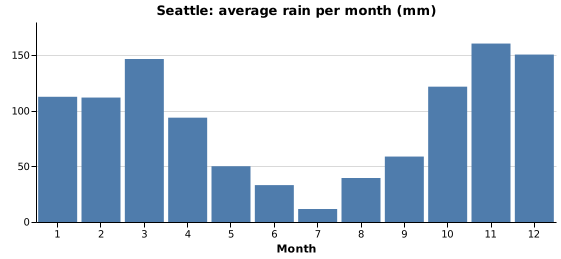
A result also has its rows as plain objects, ready for a chart. Monthly rain, from SQL to jupyter.chart:

const { rows } = await jupyter.sql`
  select month(date) as month, round(avg(precipitation) * 30, 1) as rain_mm
  from seattle group by month order by month`;
jupyter.chart({
  title: "Seattle: average rain per month (mm)",
  width: 520,
  height: 200,
  data: { values: rows },
  mark: { type: "bar", color: "#4f7cac" },
  encoding: {
    x: { field: "month", type: "ordinal", title: "Month", axis: { labelAngle: 0 } },
    y: { field: "rain_mm", type: "quantitative", title: null },
  },
});

Clean up

Closing the database frees its memory. Restarting the kernel does the same.

await jupyter.sql.close();