Have bike commutes over the Fremont Bridge come back since 2019?

NOTE

A journal Claude Code kept with the ganymede-journal plugin, shown with the outputs of its last run. The notebook, its data script and its prompts are in examples/journals/.

What the person asked

In order. The session's tool calls ran for real, driven by a script; these messages were written afterwards for the example, to show where a person steered.

1. Seattle publishes hourly bike counts for the Fremont Bridge. Have bike commutes come back since 2019? Keep a journal.
2. Is that commuters, though? Most of the bridge used to be people heading downtown in the morning.
3. Left you a note in the notebook.
4. Could 2026 just have been a dry year?
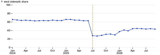
5. Finding 2 says the split stayed near 30%, but the chart climbs back to about 44% this year. And the hour chart labels its lines 2,019.

Summary.

1. Riding over the Fremont Bridge is above 2019: 3,697 riders a day from January to September 2026, +8%.
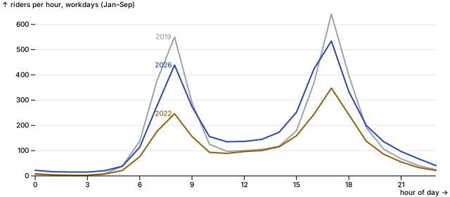
2. Commuting is not back. The 6–10 am workday window is 19% below 2019; the gain is weekends (+36%) and off-peak workday hours (midday +37%, night +34%).
3. A drier 2026 doesn't explain it: on dry days alone, weekends are +35%, workdays +1%, and the 6–10 am window is still 19% below 2019.
4. The west/east sidewalk columns change meaning on 1 Jul 2025 (west share 66% to 31% overnight, totals unchanged). Don't use them across that date.

Open: what SDOT changed on 1 Jul 2025; whether the morning gap is closing (2025 to 2026 by month); public holidays, counted here as workdays; October onward when the data is published.

Goal. Seattle counts bikes crossing the Fremont Bridge every hour, and the bridge is a main commute route from the north end to downtown and South Lake Union. Find out whether riding, and commuting in particular, is back to 2019 levels.

9 Nov 2026 · Thomas with Claude · kernel cdp-node (TypeScript, cdp-kernel 0.8.0)

Data. Hourly counts: Seattle Open Data 65db-xm6k, fetched 9 Nov 2026. Loaders are in fremont.ts next to this notebook.

Recorded: ran in the shell, not in this kernel.

$ curl -sSfo data/fremont.csv "https://data.seattle.gov/api/views/65db-xm6k/rows.csv?accessType=DOWNLOAD" && wc -l data/fremont.csv && head -2 data/fremont.csv && tail -1 data/fremont.csv

122676 data/fremont.csv
Date,"Fremont Bridge Sidewalks, south of N 34th St Total","Fremont Bridge Sidewalks, south of N 34th St Cyclist West Sidewalk","Fremont Bridge Sidewalks, south of N 34th St Cyclist East Sidewalk"
10/02/2012 01:00:00 PM,55,48,7
09/30/2026 11:00:00 PM,45,12,33

1. What does the counter cover?

Before comparing years, check which days and hours are there. A year with gaps would look like a drop in riding.

import * as pl from "npm:nodejs-polars@0.18.0";
import { hourly, daily, md } from "./fremont.ts";

const h = hourly();
const d = daily(h);
const coverage = d
  .groupBy("year")
  .agg(
    pl.col("day").count().alias("days"),
    pl.col("day").min().alias("first"),
    pl.col("day").max().alias("last"),
  )
  .join(
    h.groupBy("year").agg(pl.col("total").count().alias("hours")),
    { on: "year" },
  )
  .withColumns(pl.col("days").mul(24).minus(pl.col("hours")).alias("hours_missing"))
  .sort("year");
md(coverage)

year	days	first	last	hours	hours_missing
2012	91	2012-10-02	2012-12-31	2,171	13
2013	365	2013-01-01	2013-12-31	8,757	3
2014	365	2014-01-01	2014-12-31	8,759	1
2015	365	2015-01-01	2015-12-31	8,756	4
2016	366	2016-01-01	2016-12-31	8,783	1
2017	365	2017-01-01	2017-12-31	8,759	1
2018	365	2018-01-01	2018-12-31	8,759	1
2019	365	2019-01-01	2019-12-31	8,759	1
2020	366	2020-01-01	2020-12-31	8,783	1
2021	365	2021-01-01	2021-12-31	8,759	1
2022	365	2022-01-01	2022-12-31	8,759	1
2023	365	2023-01-01	2023-12-31	8,748	12
2024	366	2024-01-01	2024-12-31	8,783	1
2025	365	2025-01-01	2025-12-31	8,759	1
2026	273	2026-01-01	2026-09-30	6,551	1

Coverage. Every day from 2 Oct 2012 to 30 Sep 2026 is there. Each year misses one hour (the spring daylight-saving change); 2023 misses 12. No year has a gap big enough to move a yearly figure. 2026 ends on 30 Sep, so years are compared on January to September only: a full-year average would set 2026's summer against other years' winters.

2. Riders per day, by year

Average riders per day, January to September, each year against 2019.

const janSep = d.filter(pl.col("month").ltEq(9));
const byYear = janSep
  .groupBy("year")
  .agg(pl.col("total").mean().alias("per_day"))
  .sort("year");
const base2019 = byYear.filter(pl.col("year").eq(2019)).getColumn("per_day").get(0);
const yearly = byYear.withColumns(
  pl.col("per_day").div(base2019).minus(1).mul(100).alias("vs_2019_pct"),
);
md(yearly)

year	per_day	vs_2019_pct
2013	2,726	-21
2014	2,995	-13
2015	2,941	-14
2016	2,955	-14
2017	2,826	-18
2018	3,097	-10
2019	3,430	-0
2020	2,328	-32
2021	2,161	-37
2022	2,367	-31
2023	2,661	-22
2024	2,747	-20
2025	3,073	-10
2026	3,697	8

import * as Plot from "npm:@observablehq/plot@0.6.17";
import { parseHTML } from "npm:linkedom@0.18.9";
const { document } = parseHTML("<html></html>");

Plot.plot({
  document,
  width: 640,
  height: 260,
  marginLeft: 50,
  x: { label: null, tickFormat: "d" },
  y: { label: "riders per day (Jan–Sep)", grid: true },
  marks: [
    Plot.barY(yearly.toRecords(), {
      x: "year",
      y: "per_day",
      fill: (r) => (r.year === 2019 ? "#2747b8" : "#9fb0e6"),
    }),
    Plot.ruleY([base2019], { stroke: "#2747b8", strokeDasharray: "4 3" }),
    Plot.ruleY([0]),
  ],
})

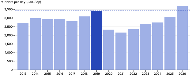
Finding 1 (revised after sections 3 to 6). Riders are back, commuters are not. January to September 2026 averages 3,697 riders a day, 8% above 2019 (3,430) and the highest since the counter started. But the gain is weekends (+36%, finding 3) and off-peak workday hours (+37% midday), while the 6–10 am commute is still 19% below 2019 (finding 4). A drier year doesn't account for it (finding 5).

3. Can the sidewalk split separate commuters? (dead end)

Thomas asked whether the gain is commuters. The counter reports the west and east sidewalks separately, and riders heading downtown in the morning favour one side, so the split looked like a proxy for direction. Before relying on it: is the split stable over time?

const split = h
  .filter(pl.col("day").gtEq(pl.lit("2024-01-01")))
  .withColumns(pl.col("day").str.slice(0, 7).alias("month_of"))
  .groupBy("month_of")
  .agg(pl.col("west").sum().div(pl.col("total").sum()).alias("west_share"))
  .sort("month_of");

Plot.plot({
  document,
  width: 640,
  height: 220,
  marginLeft: 50,
  x: { label: null },
  y: { label: "west sidewalk share", percent: true, domain: [0, 100], grid: true },
  marks: [
    Plot.lineY(split.toRecords(), { x: (r) => new Date(`${r.month_of}-01`), y: "west_share", stroke: "#2747b8", marker: "dot" }),
    Plot.ruleX([new Date("2025-07-01")], { stroke: "#94600a", strokeDasharray: "4 3" }),
  ],
})

md(
  h.filter(pl.col("day").gtEq(pl.lit("2025-06-27")).and(pl.col("day").ltEq(pl.lit("2025-07-03"))))
    .groupBy("day")
    .agg(pl.col("west").sum(), pl.col("east").sum(), pl.col("total").sum())
    .sort("day")
    .withColumns(pl.col("west").div(pl.col("total")).mul(100).alias("west_pct")),
)

day	west	east	total	west_pct
2025-06-27	2,261	1,220	3,481	65
2025-06-28	2,520	1,868	4,388	57
2025-06-29	2,325	1,900	4,225	55
2025-06-30	3,127	1,635	4,762	66
2025-07-01	1,431	3,248	4,679	31
2025-07-02	1,359	3,150	4,509	30
2025-07-03	887	2,094	2,981	30

Finding 2 (data quality). The split is not usable across 1 Jul 2025. Overnight, the west sidewalk's share fell from 66% (30 Jun) to 31% (1 Jul), while the daily total carried on unchanged (4,762 then 4,679). Riders didn't switch sides in one night: the counter or the sidewalks were reconfigured. The share stayed near 30% to the end of 2025, then rose to about 44% by spring 2026, still well below the 63–66% before the change. Totals look continuous, so the rest of this journal uses totals and time of day, not the west/east columns.

Open: confirm with SDOT what changed on 1 Jul 2025, and again in early 2026. Anyone using the west/east columns for 2025 onward will see a change in direction that didn't happen.

4. Workdays and weekends

Without direction, the next proxy is the calendar: commuting happens Monday to Friday. Average riders per day, January to September, workdays against weekends. A workday here is any Monday to Friday, public holidays included.

const kind = janSep
  .withColumns(pl.when(pl.col("workday")).then(pl.lit("workday")).otherwise(pl.lit("weekend")).alias("kind"))
  .groupBy(["year", "kind"])
  .agg(pl.col("total").mean().alias("per_day"));
const kind2019 = kind.filter(pl.col("year").eq(2019)).select("kind", pl.col("per_day").alias("base"));
const byKind = kind
  .join(kind2019, { on: "kind" })
  .withColumns(pl.col("per_day").div(pl.col("base")).minus(1).mul(100).alias("vs_2019_pct"))
  .filter(pl.col("year").gtEq(2019))
  .select("year", "kind", "per_day", "vs_2019_pct")
  .sort(["kind", "year"]);
md(byKind)

year	kind	per_day	vs_2019_pct
2019	weekend	2,035	0
2020	weekend	2,101	3
2021	weekend	1,987	-2
2022	weekend	1,985	-2
2023	weekend	1,924	-5
2024	weekend	2,026	-0
2025	weekend	2,189	8
2026	weekend	2,778	36
2019	workday	3,987	0
2020	workday	2,418	-39
2021	workday	2,230	-44
2022	workday	2,520	-37
2023	workday	2,955	-26
2024	workday	3,034	-24
2025	workday	3,427	-14
2026	workday	4,064	2

Finding 3. The gain is mostly weekends. Weekend days in 2026 average 2,778 riders, 36% above 2019; workdays average 4,064, 2% above. Workdays fell furthest (44% below 2019 in 2021) and only caught up this year.

Workdays being level doesn't mean commuting is. With hybrid work people ride at other times of day. Compare weekday hours, 2019 against now: 7–9 am is the commute.

5. Workday hours, 2019 against 2026

The cell above is Thomas's, added in JupyterLab while this ran: the daily total can hide a shift in when people ride. Average riders per hour on workdays, January to September, for 2019, 2022 (the low) and 2026. The table widens his 7–9 am to 6–10 am to take in early riders; the chart shows every hour.

const profile = h
  .filter(pl.col("month").ltEq(9).and(pl.col("workday")).and(pl.col("year").isIn([2019, 2022, 2026])))
  .groupBy(["year", "hour"])
  .agg(pl.col("total").mean().alias("riders"))
  .sort(["year", "hour"]);

Plot.plot({
  document,
  width: 640,
  height: 280,
  marginLeft: 50,
  x: { label: "hour of day", ticks: [0, 3, 6, 9, 12, 15, 18, 21] },
  y: { label: "riders per hour, workdays (Jan–Sep)", grid: true },
  color: { domain: [2019, 2022, 2026], range: ["#9aa3ad", "#94600a", "#2747b8"] },
  marks: [
    Plot.lineY(profile.toRecords(), { x: "hour", y: "riders", stroke: "year", strokeWidth: 2 }),
    Plot.text(profile.filter(pl.col("hour").eq(8)).toRecords(), { x: "hour", y: "riders", text: (r) => String(r.year), dx: -16, fill: "year" }),
    Plot.ruleY([0]),
  ],
})

const hr = pl.col("hour");
const band = pl
  .when(hr.gtEq(6).and(hr.ltEq(9))).then(pl.lit("1 morning 6–10"))
  .when(hr.gtEq(10).and(hr.ltEq(14))).then(pl.lit("2 midday 10–15"))
  .when(hr.gtEq(15).and(hr.ltEq(18))).then(pl.lit("3 evening 15–19"))
  .otherwise(pl.lit("4 night 19–6"));
const bands = h
  .filter(pl.col("month").ltEq(9).and(pl.col("workday")).and(pl.col("year").isIn([2019, 2026])))
  .withColumns(band.alias("band"))
  .groupBy(["year", "band"])
  .agg(pl.col("total").sum().alias("riders"));
const days = d.filter(pl.col("month").ltEq(9).and(pl.col("workday"))).groupBy("year").agg(pl.col("day").count().alias("n"));
const perDay = bands.join(days, { on: "year" }).withColumns(pl.col("riders").div(pl.col("n")).alias("per_day"));
const wide = perDay.filter(pl.col("year").eq(2019)).select("band", pl.col("per_day").alias("y2019"))
  .join(perDay.filter(pl.col("year").eq(2026)).select("band", pl.col("per_day").alias("y2026")), { on: "band" })
  .withColumns(pl.col("y2026").div(pl.col("y2019")).minus(1).mul(100).alias("change_pct"))
  .sort("band");
md(wide)

band	y2019	y2026	change_pct
1 morning 6–10	1,357	1,106	-19
2 midday 10–15	546	745	37
3 evening 15–19	1,587	1,544	-3
4 night 19–6	498	669	34

Finding 4. The commute has not come back; riding at other hours has. On 2026 workdays the 6–10 am window carries 1,106 riders, 19% fewer than in 2019 (1,357), and the 3–7 pm window is 3% lower. Midday (+37%) and night (+34%) make up the difference. The workday total matches 2019 only because trips moved out of the peaks.

Recorded: ran in the shell, not in this kernel.

$ curl -sSfo data/seatac.csv "https://www.ncei.noaa.gov/access/services/data/v1?dataset=daily-summaries&stations=USW00024233&startDate=2012-10-01&endDate=2026-09-30&dataTypes=PRCP,TMAX&format=csv&units=metric" && wc -l data/seatac.csv && head -2 data/seatac.csv

5114 data/seatac.csv
"STATION","DATE","PRCP","TMAX"
"USW00024233","2012-10-01","0.0","23.3"

6. Was 2026 just a dry year?

Thomas asked whether weather explains it: a dry year would lift weekend and midday riding most. SeaTac daily rain (NOAA GHCN-Daily, station USW00024233, fetched 9 Nov 2026 by the recorded command above). A day with 1 mm of rain or more counts as wet. Compare the wet-day share by year, then the same splits on dry days only: workdays against weekends, and the workday hour bands from section 5.

import { weather } from "./fremont.ts";
const wx = weather();
const dw = janSep.join(wx, { on: "day" }).withColumns(pl.col("rain_mm").gtEq(1).alias("wet"));

const wetShare = dw
  .filter(pl.col("year").isIn([2019, 2022, 2025, 2026]))
  .groupBy("year")
  .agg(pl.col("wet").mean().mul(100).alias("wet_days_pct"), pl.col("tmax_c").mean().alias("avg_high_c"))
  .sort("year");
md(wetShare, 1)

year	wet_days_pct	avg_high_c
2019	31.9	17.9
2022	25.6	17.2
2025	22.7	17.8
2026	23.8	17.9

const dry = dw
  .filter(pl.col("wet").not().and(pl.col("year").isIn([2019, 2026])))
  .withColumns(pl.when(pl.col("workday")).then(pl.lit("workday")).otherwise(pl.lit("weekend")).alias("kind"))
  .groupBy(["kind", "year"])
  .agg(pl.col("total").mean().alias("per_dry_day"), pl.col("day").count().alias("days"))
  .sort(["kind", "year"]);
md(dry)

kind	year	per_dry_day	days
weekend	2019	2,322	57
weekend	2026	3,124	61
workday	2019	4,474	129
workday	2026	4,540	147

const dryDays = dw.filter(pl.col("wet").not().and(pl.col("workday"))).select("day");
const dryBands = h
  .join(dryDays, { on: "day" })
  .filter(pl.col("year").isIn([2019, 2026]))
  .withColumns(band.alias("band"))
  .groupBy(["year", "band"])
  .agg(pl.col("total").sum().alias("riders"))
  .join(dryDays.join(d, { on: "day" }).groupBy("year").agg(pl.col("day").count().alias("n")), { on: "year" })
  .withColumns(pl.col("riders").div(pl.col("n")).alias("per_day"));
md(
  dryBands.filter(pl.col("year").eq(2019)).select("band", pl.col("per_day").alias("y2019"))
    .join(dryBands.filter(pl.col("year").eq(2026)).select("band", pl.col("per_day").alias("y2026")), { on: "band" })
    .withColumns(pl.col("y2026").div(pl.col("y2019")).minus(1).mul(100).alias("change_pct"))
    .sort("band"),
)

band	y2019	y2026	change_pct
1 morning 6–10	1,492	1,209	-19
2 midday 10–15	626	844	35
3 evening 15–19	1,777	1,738	-2
4 night 19–6	578	749	29

Finding 5. Weather doesn't explain it. 2026 was drier than 2019 (24% of days wet against 32%), but on dry days alone the pattern holds: weekends 3,124 riders against 2,322 (+35%), workdays 4,540 against 4,474 (+1%). On dry workdays the hour bands match finding 4: the 6–10 am window is 19% below 2019, midday +35%, night +29%.